01: Overview

VAEs are the Rosetta Stone between “classical” latent-variable models and the modern generative zoo—diffusion, EBMs, JEPA, world models all inherit pieces of this logic, even when they loudly deny it.

Let’s walk this in a systematic, model-builder’s way, using the screenshot as our concrete anchor rather than a fog of abstractions.

1. What problem a VAE is actually solving¶

At heart, a VAE is doing approximate Bayesian inference in a latent-variable model.

We posit a generative story:

Sample a latent variable \(z \sim p(z)\), usually \(\mathcal{N}(0, I)\)
Generate data \(x \sim p_\theta(x \mid z)\)

This defines a joint distribution:

\[ p_\theta(x, z) = p_\theta(x \mid z) \cdot p(z) \]

What we want is the marginal likelihood:

\[ p_\theta(x) = \int p_\theta(x \mid z) p(z) \, dz \]

That integral is the villain of the story. Deep nets make it intractable.

2. Variational inference: replacing the impossible with the trainable¶

Enter the encoder—not as a compression device, but as an approximate posterior:

\[ q_\phi(z \mid x) \approx p_\theta(z \mid x) \]

Instead of solving Bayes’ rule exactly, we learn a distribution that’s close.

This gives us the ELBO (Evidence Lower Bound):

\[ \log p_\theta(x) \geq \underbrace{\mathbb{E}_{q_\phi(z|x)}[\log p_\theta(x|z)]}_{\text{reconstruction}} - \underbrace{\mathrm{KL}(q_\phi(z|x) \| p(z))}_{\text{regularization}} \]

This equation is the soul of the VAE. Everything in your screenshot is just bookkeeping around this identity.

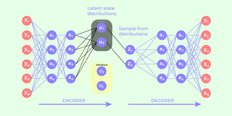
3. Why the encoder outputs μ and σ, not a point¶

A deterministic autoencoder learns:

\[ x \mapsto z \mapsto \hat{x} \]

A VAE learns:

\[ x \mapsto (\mu(x), \sigma(x)) \Rightarrow q_\phi(z \mid x) \]

Usually:

\[ q_\phi(z \mid x) = \mathcal{N}(\mu(x), \text{diag}(\sigma^2(x))) \]

This matters because:

We are learning a distribution over latent causes, not a code
The KL term forces this distribution to stay near the prior
Sampling becomes meaningful: different \(z\)'s produce different but plausible \(x\)'s

Your screenshot’s green (\(\mu\)) and purple (\(\sigma\)) blocks are not decoration—they are the model.

4. The reparameterization trick: making randomness differentiable¶

Sampling is not differentiable:

\[ z \sim \mathcal{N}(\mu, \sigma^2) \]

So we rewrite it as:

\[ \epsilon \sim \mathcal{N}(0, I), \quad z = \mu + \sigma \odot \epsilon \]

Now:

Randomness is isolated in \(\epsilon\)
\(\mu\) and \(\sigma\) are deterministic functions of \(x\)
Gradients flow cleanly through the graph

This is why the trick is not a hack—it’s a change of variables.

In your screenshot, the blue ε block feeding into \(\mu + \epsilon \odot \sigma\) is the mathematical pivot that makes VAEs trainable.

5. Why the KL term has that closed form¶

Because both distributions are Gaussians:

\[ q_\phi(z|x) = \mathcal{N}(\mu, \sigma^2), \quad p(z) = \mathcal{N}(0, I) \]

The KL divergence reduces to:

\[ \mathrm{KL} = \frac{1}{2} \sum_{i=1}^{d} \left( \mu_i^2 + \sigma_i^2 - \log \sigma_i^2 - 1 \right) \]

This term:

Penalizes large means (keeps latent centered)
Penalizes tiny variances (prevents memorization)
Encourages smooth, well-filled latent space

This is why VAEs interpolate nicely but look blurry: you’re paying for continuity with entropy.

6. Decoder: likelihood, not reconstruction “error”¶

One subtle but crucial point:

The decoder defines a likelihood model, not just a pixel predictor.

Examples:

Bernoulli → binary images
Gaussian → continuous data
Categorical → tokens

So the reconstruction term is:

\[ \mathbb{E}_{q(z|x)}[\log p_\theta(x \mid z)] \]

Mean squared error is just one special case of a Gaussian likelihood with fixed variance.

7. Conditional VAE (cVAE): controlled generation¶

Now we add a condition \(y\):

Generative story:

\[ z \sim p(z), \quad x \sim p_\theta(x \mid z, y) \]

Inference:

\[ q_\phi(z \mid x, y) \]

ELBO:

\[ \mathbb{E}_{q(z|x,y)}[\log p_\theta(x|z,y)] - \mathrm{KL}(q(z|x,y) \| p(z)) \]

Practically:

Concatenate \(y\) to encoder input
Concatenate \(y\) to decoder input
Sampling with fixed \(y\) gives conditional generation

This is the conceptual ancestor of classifier-free guidance in diffusion.

8. Mental model: what VAEs get right—and wrong¶

VAEs give you:

Explicit latent variables
Amortized inference
A proper probabilistic objective
A bridge between Bayesian models and deep nets

They struggle with:

Sharp details (entropy pressure)
Expressive posteriors (Gaussian bottleneck)
Multi-modal likelihoods

Which is why the field evolved toward:

Diffusion (score matching instead of likelihood)
EBMs / JEPA (implicit densities, no decoder likelihood)
World models (latent dynamics + control)

9. How this connects forward to your roadmap¶

You can think of modern generative models as VAEs that rebelled:

Diffusion: remove decoder likelihood, learn score instead
EBMs / JEPA: drop explicit density, learn energy or invariants
World models: put dynamics inside the latent space
Flow matching: continuous reparameterization without KL

But the core tension—latent structure vs tractability—starts here.

Suggested next step (logical, not trendy)¶

Before jumping to diffusion, a powerful intermediate stop is:

β-VAE (disentanglement vs capacity)
IWAE (tightening the ELBO)
VAE with learned priors (VampPrior)

Those sharpen your intuition for why diffusion took over—and what it sacrificed.

When you’re ready, we can deliberately “break” the VAE and watch diffusion emerge from the wreckage.

10. References & Further Reading¶

Foundational Papers¶

Kingma & Welling (2014) — "Auto-Encoding Variational Bayes" — The original VAE paper
Rezende et al. (2014) — "Stochastic Backpropagation and Approximate Inference in Deep Generative Models"
Sohn et al. (2015) — "Learning Structured Output Representation using Deep Conditional Generative Models" — cVAE

VAE Variants¶

Higgins et al. (2017) — "β-VAE: Learning Basic Visual Concepts with a Constrained Variational Framework"
Burda et al. (2016) — "Importance Weighted Autoencoders" (IWAE)
Tomczak & Welling (2018) — "VAE with a VampPrior"

Bridge to Diffusion¶

Cao et al., "A Survey on Generative Diffusion Models" (2024) — Comprehensive treatment of score matching and diffusion
Song & Ermon (2019) — "Generative Modeling by Estimating Gradients of the Data Distribution"
Ho et al. (2020) — "Denoising Diffusion Probabilistic Models" (DDPM)

Biology Applications¶

Lopez et al. (2018) — "Deep generative modeling for single-cell transcriptomics" (scVI)
Lotfollahi et al. (2019) — "scGen: Predicting single-cell perturbation responses"

Learning Roadmap¶

See ROADMAP.md for the full progression from VAE → Diffusion → EBMs → JEPA → World Models.