VAE Model Training: Interpreting Loss Curves and Diagnostics¶

This document explains how to interpret VAE training output, diagnose common issues like posterior collapse, and understand the interplay between reconstruction and KL divergence.

The ELBO Loss¶

VAEs maximize the Evidence Lower Bound (ELBO), or equivalently minimize the negative ELBO:

\[ \mathcal{L} = \underbrace{-\mathbb{E}_{q(z|x)}[\log p(x|z)]}_{\text{reconstruction loss}} + \underbrace{\text{KL}(q(z|x) \| p(z))}_{\text{regularization}} \]

In practice, with a β-VAE formulation:

\[ \mathcal{L} = \mathcal{L}_{\text{recon}} + \beta \cdot \mathcal{L}_{\text{KL}} \]

where:

Reconstruction loss: How well the decoder reconstructs the input (MSE for Gaussian, NLL for NB/ZINB)
KL divergence: How much the learned posterior \(q(z|x)\) deviates from the prior \(p(z) = \mathcal{N}(0, I)\)
β: Weight controlling the trade-off (β = 1 is standard VAE, β > 1 encourages disentanglement)

Interpreting Training Output¶

A typical training log looks like:

epoch 001 | train loss=0.8684 recon=0.8440 kl=0.0488 | val loss=0.7531
epoch 005 | train loss=0.5926 recon=0.4825 kl=0.2203 | val loss=0.5779
epoch 010 | train loss=0.5083 recon=0.3807 kl=0.2554 | val loss=0.4987
epoch 018 | train loss=0.4374 recon=0.2755 kl=0.3238 | val loss=0.4253

What Each Metric Means¶

Metric	Formula	Interpretation
loss	recon + β × kl	Total objective (lower = better)
recon	MSE or NLL	Reconstruction quality
kl	KL(q \|\| p)	Information encoded in latent space

Healthy Training Signs¶

Total loss decreasing — The model is learning
Reconstruction improving — The decoder is getting better
KL increasing then stabilizing — The latent space is being used
Train ≈ Val — No significant overfitting

The KL Term: Why It Matters¶

What KL Measures¶

The KL divergence measures how different the learned posterior \(q_\phi(z|x)\) is from the prior \(p(z) = \mathcal{N}(0, I)\).

\[ \text{KL}(q(z|x) \| p(z)) = \frac{1}{2} \sum_{j=1}^{d} \left( \mu_j^2 + \sigma_j^2 - \log \sigma_j^2 - 1 \right) \]

where \(\mu_j\) and \(\sigma_j\) are the encoder outputs for latent dimension \(j\).

Interpreting KL Values¶

KL Value	What It Means
≈ 0	Posterior equals prior — encoder ignores input
0.1 – 1.0	Healthy range — latent encodes meaningful variation
> 2.0	Posterior far from prior — may indicate underfitting or need for higher β

Posterior Collapse: The KL ≈ 0 Problem¶

What Is Posterior Collapse?¶

When \(\text{KL}(q(z|x) \| p(z)) \approx 0\), it means:

\[ q_\phi(z|x) \approx p(z) = \mathcal{N}(0, I) \quad \text{for all } x \]

This looks mathematically fine, but the problem is: the encoder outputs the same distribution regardless of the input.

Why It's Bad¶

If \(q(z|x) \approx \mathcal{N}(0, I)\) for all inputs:

The encoder has learned to ignore the input
Every sample maps to roughly the same latent distribution
The latent code \(z\) carries no information about \(x\)
The latent space is useless for downstream tasks

Why It Happens¶

The decoder becomes so powerful that it can reconstruct \(x\) without using \(z\). It essentially memorizes the data distribution.

The model finds an "easy" solution: minimize KL by setting \(q(z|x) = p(z)\), and let the decoder do all the work.

How to Detect It¶

Symptom	Healthy	Collapsed
KL during training	Increases, then stabilizes (0.1–1.0)	Stays near 0
Latent space (UMAP)	Clusters by meaningful factors	All points in one blob
Downstream classification	Good accuracy	Near random

How to Fix It¶

Lower β — Reduce KL penalty (e.g., β = 0.1 or 0.5)
KL annealing — Start with β = 0, gradually increase
Free bits — Allow minimum KL per dimension before penalizing
Weaker decoder — Reduce decoder capacity
Cyclical annealing — Periodically reset β to 0

The β Parameter¶

Effect of Different β Values¶

β Value	Effect
β < 1	Prioritize reconstruction, allow higher KL
β = 1	Standard VAE (balanced)
β > 1	Prioritize regularization, encourage disentanglement

Practical Guidance¶

Start with β = 0.5 for gene expression data
If KL stays near 0, reduce β further
If reconstruction is poor, reduce β
If latent space is unstructured, increase β

KL Annealing¶

A common technique to avoid posterior collapse:

def kl_annealing_schedule(epoch, warmup_epochs=10, max_beta=1.0):
    """Linear KL annealing."""
    return min(max_beta, max_beta * epoch / warmup_epochs)

This allows the model to first learn good reconstructions, then gradually enforce the prior constraint.

Example: Healthy Training Curves¶

The figure below shows training curves from a cVAE trained on synthetic bulk RNA-seq data (notebooks/vae/01_bulk_cvae.ipynb):

Healthy VAE Training Curves

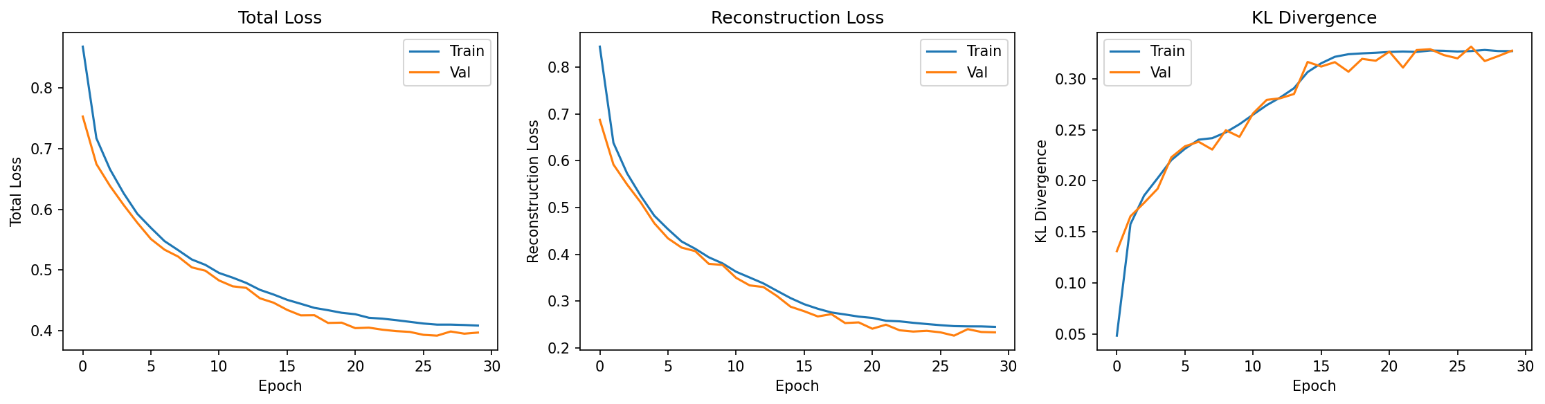
What to observe:

Total Loss (left): Both train and val decrease smoothly, converging together
Reconstruction Loss (center): Decreases rapidly early, then plateaus — the decoder is learning
KL Divergence (right): Increases from ~0.05 to ~0.32, then stabilizes — the latent space is being used

This is a textbook example of healthy VAE training: good reconstruction, no posterior collapse, no overfitting.

Example: Diagnosing Your Training¶

Given this output:

epoch 001 | recon=0.84 kl=0.05
epoch 010 | recon=0.38 kl=0.26
epoch 018 | recon=0.28 kl=0.32

Diagnosis:

✅ Reconstruction improving (0.84 → 0.28)
✅ KL increasing (0.05 → 0.32) — latent space is being used
✅ KL in healthy range (0.1–1.0)
✅ No posterior collapse

Conclusion: Training is healthy. The model is learning meaningful latent representations.

Summary¶

Metric	Want to See	Red Flag
Total loss	Decreasing, train ≈ val	Diverging train/val
Reconstruction	Decreasing	Stuck high
KL	Increases then stabilizes (0.1–1.0)	Stays near 0

The key insight: KL ≈ 0 means the latent space is useless, even though it technically satisfies the prior constraint. A healthy VAE has moderate KL, indicating the encoder is learning to compress input-specific information into the latent space.